Inverse Transform Sampling

Published: 2023-06-24

Inverse transform sampling is a basic method for pseudo-random number generation. It can be used for the generation of random samples from a non-uniform probability distribution, when its cumulative distribution function is known.

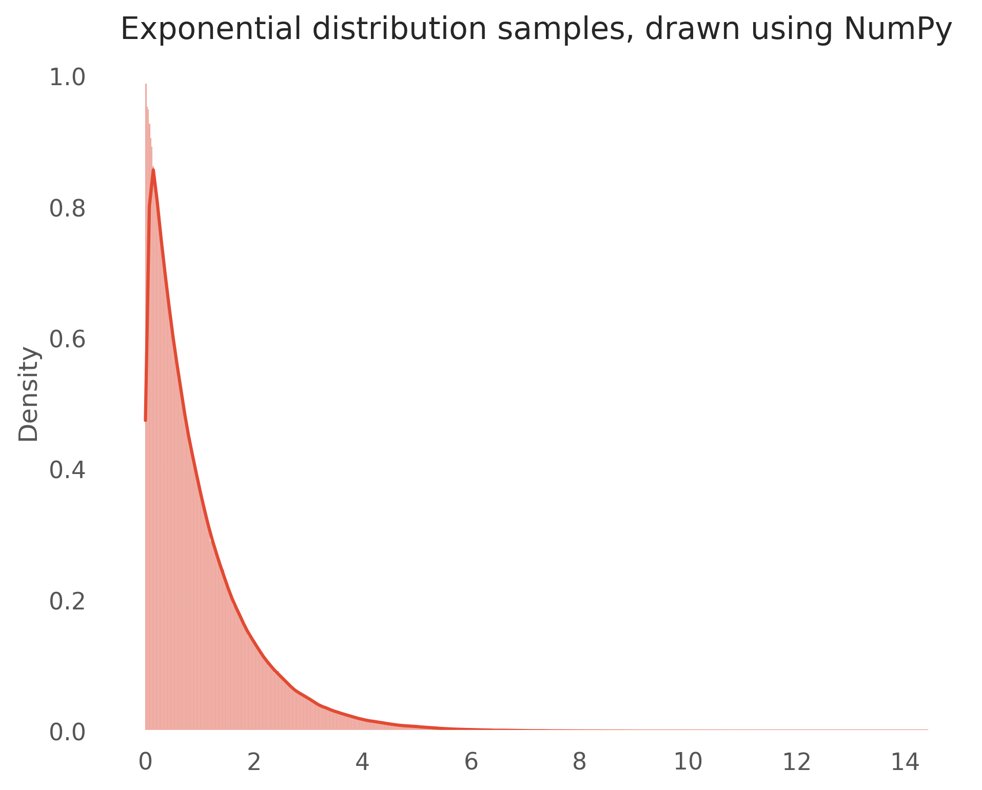
The main idea of inverse transform sampling is quite simple. We want to sample from a non-uniform distribution by mapping a sampled point from a uniform distribution $U[0,1]$ , to the inverse cumulative distribution function (CDF) of the non-uniform distribution. To understand how it works, let’s consider the exponential distribution as an example. This post will demonstrate how inverse transform sampling done programmatically using Python. Before we delve into the implementation, let’s first use an existing library to sample from the exponential distribution for comparison purposes. In this case, we will sample $10^6$ points from the exponential distribution using the Numpy library:

import numpy as np
import seaborn as sns

# sample from exponential distribution using numpy
exponential_sample = np.random.exponential(scale=1.0, size=[int(1e6)])
# plotting
sns.displot(exponential_sample, kde=True, stat="density")

PDF of exponential distribution is $f(x) = e^{-\lambda x}$ , with $x>0$ . The CDF is the integral of its PDF, thus the CDF is defined as:

$F(x) = 1-e^{- \lambda x}$

using simple algebra, the inverse takes the following form:

$F^{-1}(u) = \frac{- \log(1-u)}{\lambda}$

we can then do the inverse transform sampling as follows:

# define the inverse CDF function of exponential distributin
def exp_cdf_inv(u, scale=1):
  return - np.log(1-u)/scale

# sample 1e6 points uniformly
uniform_sample = np.random.uniform(size=[int(1e6)])

# map the sampled points using inverse CDF of exponential distribution
inverse_transform_exponential = exp_cdf_inv(uniform_sample)

# plotting
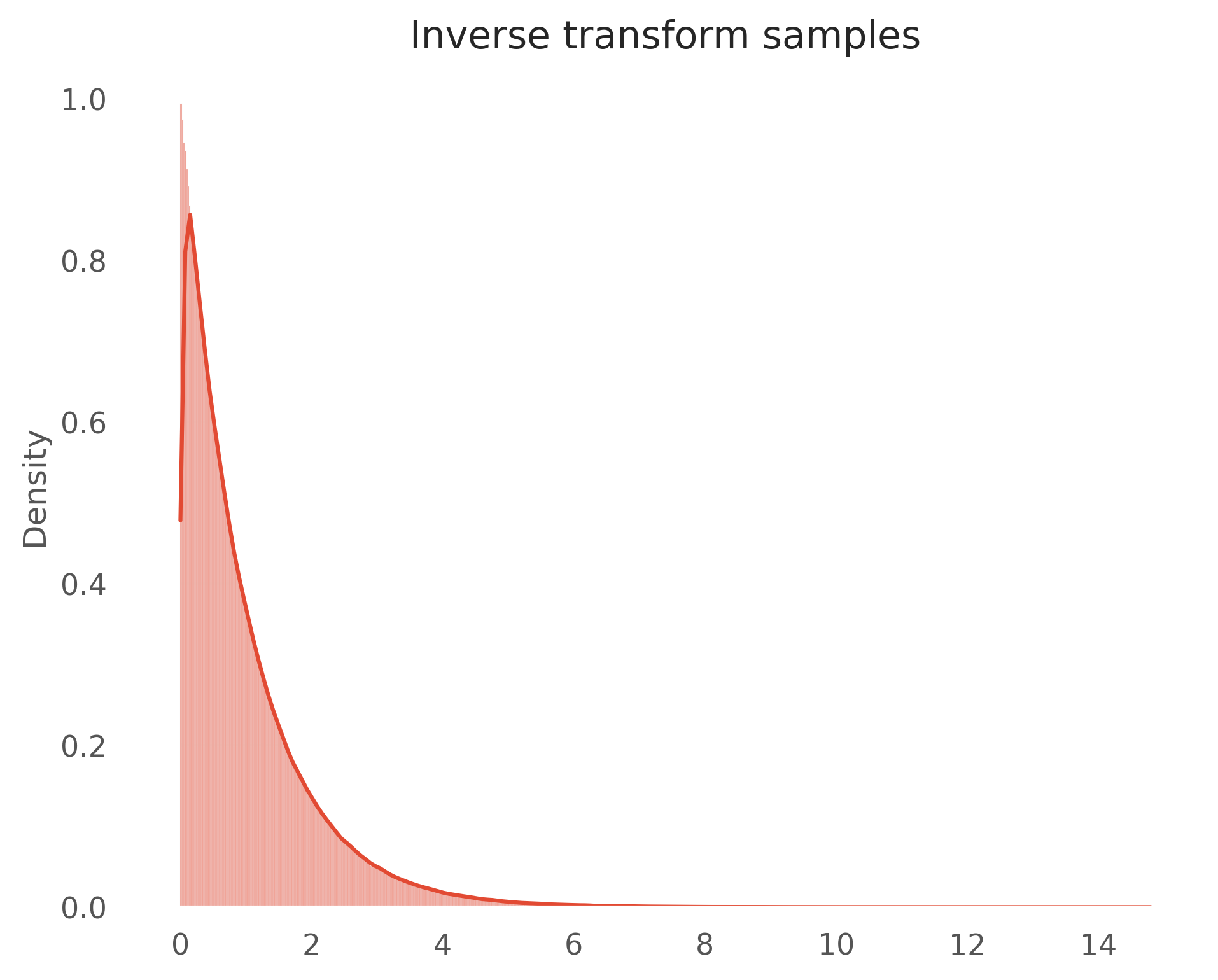
sns.displot(inverse_transform_exponential, kde=True, stat="density");

As we can see from the picture above, we got very similar result compared to the Numpy’s implementation!

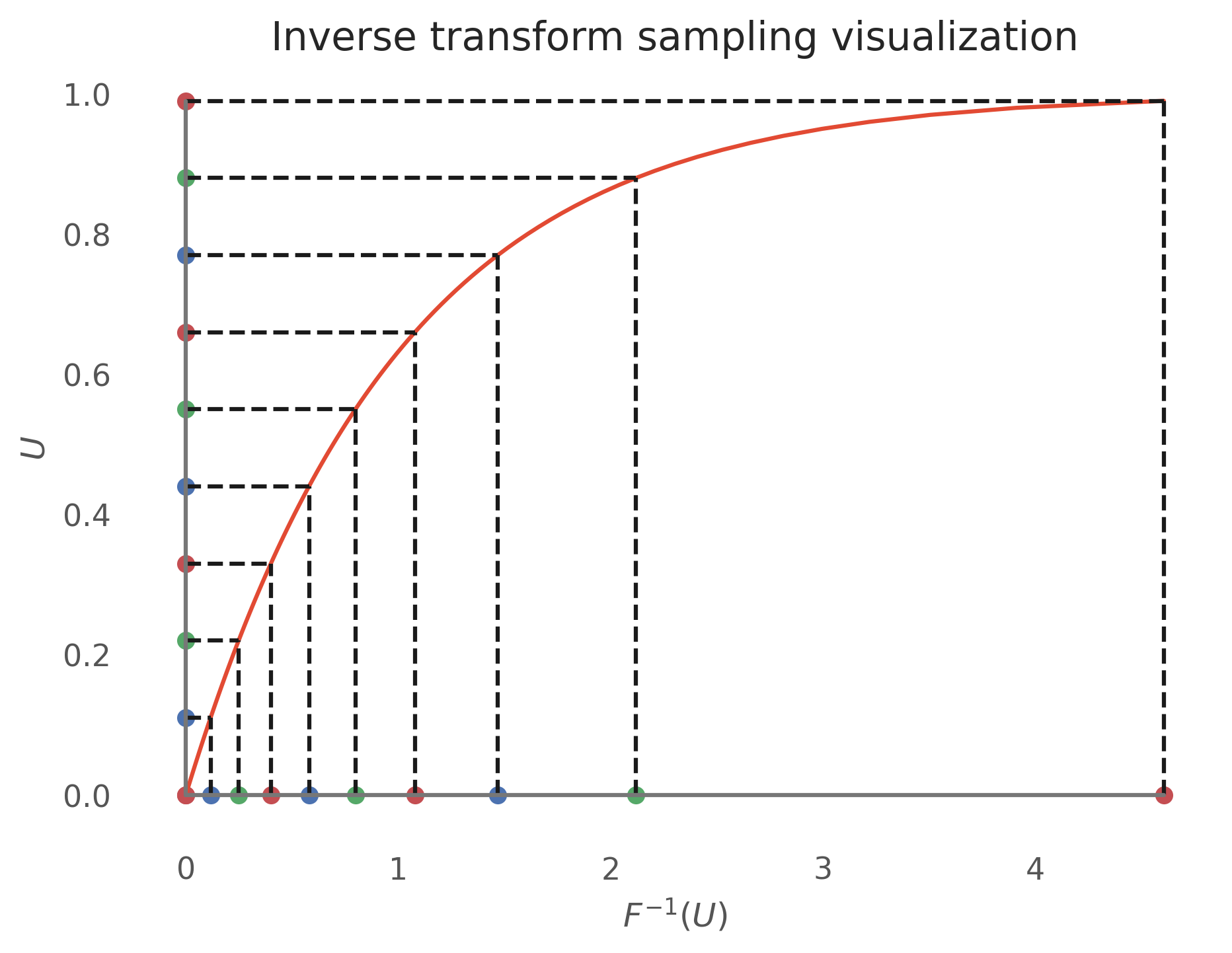
To better grasp the intuition of this inverse transform sampling, Let’s visualize the mapping from the uniform points to the exponential distribution using the inverse CDF. In this case, we will examine the same evenly spaced points to observe how the distances between points are altered by the inverse CDF.

import itertools

fig, ax = plt.subplots(figsize=(7,5))

n_points = 10

ax.plot(exp_cdf_inv(np.arange(0,1,0.01)), np.arange(0,1,0.01))
ax.stem(np.linspace(0,0.99,n_points), exp_cdf_inv(np.linspace(0,0.99,n_points)),
		linefmt="k--", orientation="horizontal", markerfmt="none")
ax.stem(exp_cdf_inv(np.linspace(0,0.99,n_points)), np.linspace(0,0.99,n_points),
		linefmt="k--",markerfmt="none")

def plot_rainbow(xs,ys):
  colors = itertools.cycle(["r", "b", "g"])
  for x,y in zip(xs,ys):
      plt.scatter(x, y, color=next(colors))

plot_rainbow(exp_cdf_inv(np.linspace(0,0.99,n_points)),np.zeros(n_points))
plot_rainbow(np.zeros(n_points),np.linspace(0,0.99,n_points))

ax.set_xlabel("$F^{-1}(U)$")
ax.set_ylabel("$U$")

The y-axis above is the uniform point on $[0,1]$ domain, and the x-axis is the inverse CDF of the exponential distribution with scale $\lambda = 1$ . Notice that as the uniform points approach 0, the density becomes increasingly concentrated in that region. This behavior is expected for the exponential distribution with a scale parameter of $\lambda = 1$ .

Inverse Transform Sampling

References: